Things to do better next time

I have had some errors found in my assembled transcriptomes when they were submitted to NCBI. It appears that I missed a couple of quality control steps at the trimming stage.

What I have learnt:

• after using the default trimmomatic settings – check the data before proceeding.
• incorporate a file with all Illumina primers for identifying and trimming these from reads.
• use bbduk to help with this process – as other residual primers may be there – from previous runs on the machine (http://jgi.doe.gov/data-and-tools/bbtools/bb-tools-user-guide/bbduk-guide/).
• screen the raw data for contaminants, eg. bacterial, human and other non-target sequences. Seems my transcriptomes included a  few sequences from humans, gorilla and chimp!!
• None of this really affected my analysis and, in fact, was such a small proportion of the assembled transcriptome BUT – the assemblies are now a bit questionable and should be done again.

Finally to get the counts

Now with all the bam files, indexed bam files and the bed file made previously we can get read counts per transcript. The moment you are anticipating is not far off. Make sure the bam.bai files are all in the same working directory.

We use BEDtools v2.24.0, with the multiBamCov option.

#PBS -P project
#PBS -N Syzygium_counts
#PBS -l nodes=1:ppn=20
#PBS -l walltime=01:00:00
#PBS -l pmem=24gb
#PBS -e ./Syzygium_counts.txt
#PBS -M email@sydney.edu.au
#PBS -m abe

# Load modules
module load bedtools

# Working directory
cd /working directory location

# Run bedtools script
multiBamCov -q 30 -p -bams AP0_coordSorted.bam AP1_coordSorted.bam AP2_coordSorted.bam -bed Syzygium.BED > Syzygium_counts.txt

The output from this will be a large text file with the numbers of reads that aligned to each transcript.

TRINITY_DN4630_c0_g1_i1 0 2449 68 0 18 30
TRINITY_DN4630_c0_g2_i1 0 457 2 0 4 4 0
TRINITY_DN4679_c0_g1_i1 0 410 2 0 2 0 0
TRINITY_DN4674_c0_g1_i1 0 227 4 0 0 0 0
TRINITY_DN4609_c0_g1_i1 0 265 0 0 0 0 0
TRINITY_DN4651_c0_g1_i1 0 1030 8 0 4 4

which you can put into a spreadsheet and name the columns. And the columns are in the order that the bam files are placed in the script. Of course you would include all the bam files for all samples and all times in the one run using bedtools.

Gene ID	start	end	AP0	AP1	AP2
TRINITY_DN4630_c0_g1_i1	0	2449	68	0	18
TRINITY_DN4630_c0_g2_i1	0	457	2	0	4
TRINITY_DN4679_c0_g1_i1	0	410	2	0	2
TRINITY_DN4674_c0_g1_i1	0	227	4	0	0
TRINITY_DN4609_c0_g1_i1	0	265	0	0	0
TRINITY_DN4651_c0_g1_i1	0	1030	8	0	4

Running biopython scripts

As I am learning a bit about scripts and how to run them I have made recent errors which probably appear very simple to someone from a computing background.

The word I have learnt is ‘parse‘ which means:

• to analyze (a sentence) into its parts and describe their syntactic roles.
• analyze (a string or text) into logical syntactic components, typically in order to test conformability to a logical grammar.
• examine or analyze minutely.

Another word is to ‘pass‘. You pass some instruction to the software to parse (analyze).

To run software you need:

• the software and dependencies (other software) to be installed
• script to tell the program what you want it to do
• input files

I managed to find this very useful biopython script to make bed files from my newly made transcriptomes. Bed files are tab  delimited files that include the sequence ID, and the start and end location. For new transcriptomes the start is always 0 and the end is the length of the contig. These files can be used to gather the count data from your alignment files per sequence ID (gene).

http://ged.msu.edu/angus/tutorials-2013/rnaseq_bwa_counting.html

In case the website above is unavailable, here is the biopython script, slightly altered for the later version of Biopython which requires brackets around the print function:

import sys
from Bio import SeqIO

fasta_handle = open(sys.argv[1], "rU") #Open the fasta file specified by the user on the command line

#Go through all the records in the fasta file
for record in SeqIO.parse(fasta_handle, "fasta"):
    cur_id = record.id #Name of the current feature
    cur_length = len(record.seq) #Size of the current feature
    print (("%s\t%d\t%d") % (cur_id, 0, cur_length)) #Output the name, start, and end coordinates to the screen

This script will take any fasta file you give it and output the bed file. The important thing is to tell python.exe what to do with the input file. You need to pass the script to python.exe so it can parse and act on it. Therefore the order of your command must be correct – the .py script comes directly after the python.exe.

I placed the input file first and could not understand why I kept getting the error that my fasta file had syntax errors.

So in the command line window – I just run this in Windows cmd.exe by holding shift and right-clicking on the folder I want as my working directory;

Open the command window in the directory where your fasta file is, then input the directory path to Python34\python.exe then input the directory path to the script and output to your working directory.

So it will look something like this:

D:\Syzygium\>C:Python34\python.exe D:\scripts\make_bed_from_fasta.py Syzygium.fasta > Syzygium.bed

The output will look like this showing the length of each ‘gene’.

TRINITY_DN4638_c0_g1_i1 0 486
TRINITY_DN4638_c0_g2_i1 0 486
TRINITY_DN4608_c0_g1_i1 0 442
TRINITY_DN4687_c0_g1_i1 0 207
TRINITY_DN4630_c0_g1_i1 0 2449
TRINITY_DN4630_c0_g2_i1 0 457
TRINITY_DN4679_c0_g1_i1 0 410
TRINITY_DN4674_c0_g1_i1 0 227
TRINITY_DN4609_c0_g1_i1 0 265
TRINITY_DN4651_c0_g1_i1 0 1030
TRINITY_DN4626_c0_g1_i1 0 468
TRINITY_DN4626_c1_g1_i1 0 286
TRINITY_DN4653_c0_g2_i1 0 555
TRINITY_DN4653_c1_g1_i1 0 793
TRINITY_DN4648_c0_g1_i1 0 605
TRINITY_DN4632_c0_g1_i1 0 2026
TRINITY_DN4672_c0_g1_i1 0 239

 

Clustering the transcriptomes

I have now made eight transcriptomes. Four from the resistant plants and four from the susceptible. To be able to compare expression from different times, and between the different biological replicates, I have to make a single transcriptome for the plant species, in this case, Syzygium (Lilly Pilly). This is a bit concerning as my plants are grown from wild sourced seeds and are likely to be highly heterozygous.

My approach therefore was to use the CD-HIT-EST-2D (http://weizhongli-lab.org/cd-hit/) software to combine transcriptomes, initially at 0.95  similarity. I clustered the transcriptomes in pairs from the largest to the smallest until I had a single fasta file.

#PBS -P (project)
#PBS -N SYZ1_CD-HIT
#PBS -l nodes=1:ppn=20
#PBS -l walltime=00:15:00
#PBS -l pmem=24gb
#PBS -e ./SYZ1.error
#PBS -M (email address)
#PBS -m abe

# Load modules
module load cd-hit/4.6.1

# Working directory
Input path to directory

# Run CD-Hit script
cd-hit-est-2d -i BU.fasta -i2 BS.fasta -o SYZ1.fasta -c 0.95 -n 10 -d 0 -M 0 -T 0

I then sought out highly conserved genes using local BLAST in BioEdit. I used a couple of Eucalyptus grandis chitinase genes that I know to be well conserved from previous work, currently under review.

I found that the genes were present and intact in the individual transcriptomes but not in the combined one. I therefore ran the process with CD-HIT again with a higher stringency of 0.98.

This time the genes were present in the final transcriptome making me feel more confident about the alignment process.

Building the transcriptome

The purpose of many RNAseq studies is to compare the gene expression patterns across different treatments. In order to do this, as I mentioned in the previous post, all the reads from each treatment (from the one plant) need to be combined first.

Trinity assembly software incorporates other tools as well as assembly, for example Trimmomatic can be run within the trinity pipeline. To do the trimming and assembly you would run a script like this (note no spaces or line breaks):

Trinity –seqType fq –max_memory 24G –CPU 7 –left AP0_R1.fastq,AP1_R1.fastq,AP2_R1.fastq –right AP0_R2.fastq,AP1_R2.fastq,AP2_R2.fastq–trimmomatic –output AP_trinity

This will build all the reads into a complete transcriptome for the plant labelled AP from RNA expressed pre-inoculation, at 24 hours and at 48 hours.

Depending on the success of the sequencing, ie. the number and length of raw reads, the assembly process will take around 1 to 3 days of wall-time. Below is the pbs script to run for trimmed reads.

#PBS -P (project name)
#PBS -N AP_assembly
#PBS -l nodes=1:ppn=24
#PBS -l walltime=100:00:00
#PBS -l pmem=24gb
#PBS -e ./AP_trinity/AP_assembly.txt
#PBS -M email@sydney.edu.au
#PBS -m abe

# Load modules
module load bowtie
module load java
module load trinity/2.1.1

# Working directory
cd /project/full path name to your working directory (where all the input files are)

# Run trinity
Trinity –seqType fq –max_memory 24G –CPU 24 –left AP0_R1.trimpaired.fastq,AP1_R 1.trimpaired.fastq,AP2_R1.trimpaired.fastq –right AP0_R2.trimpaired.fastq,AP1_R2.trimpaired.fastq,AP2_R2.trimpaired.fastq –output AP_trinity

NB: As I said previously, I am learning on the process as I go. Actually writing this bog is making me find the mistakes I have made along the way. Just found an error in the way I ran the above trinity script. It appears that the paired and unpaired trimmed reads are combined with the trinity assembly. I have only used my paired reads. At this point I am way down the pipeline so this is a big blow! I have decided to continue with my current pipeline as well as re-run the assemblies with both the paired and un-paired reads and then compare the outcomes.

Why do RNAseq?

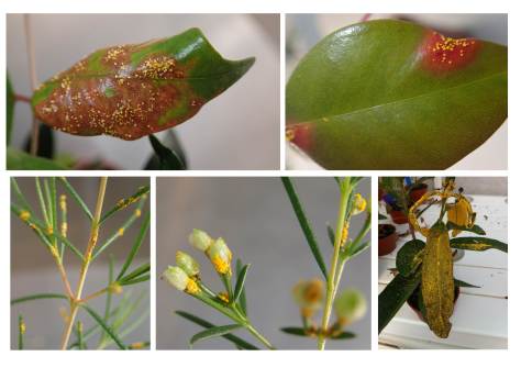
There is always a scientific question at the basis of doing RNAseq. Here are some images of susceptible Myrtaceae plants infected with myrtle rust. Clockwise from top left: Syzygium luehmannii (Riberry), Syzygium leuhmannii, Syzygium jambos, Chamelaucium uncinatum (Geraldton wax) flower buds, Chamelaucium uncinatum stems and leaves. For highly susceptible plants the pathogen can be devastating. Determining the genetic basis for resistance would therefore be very useful for plant breeding and for population and species management. Whole gene expression studies are one way to determine this genetic basis by identifying the changes in resistant versus susceptible plants.

 

Trinity assembly – and how not to go about it

I have used the Trinity assembly software to build denovo transcriptomes for each of my plants. Lots of good information here:

https://github.com/trinityrnaseq/trinityrnaseq/wiki

I made several errors to begin with. The first error was to build transcriptomes for each plant at each time-point thinking that this would allow me to compare across the treatments. Running the assembly software can take days to complete – so this has meant a lot of time wasted doing 24 separate assemblies!

The correct thing to do is to combine the data from all times (pre-inoculation, 24 hours post-inoculation and 48 hours post-inoculation) for each plant. In my case I did 8 assemblies. You need all the gene transcripts from all samples to build the most complete ‘potential’ expression profile. You can then use this transcriptome fasta file to map the reads from each treatment later on. The transcriptome is also really useful for other analysis you might want to do later such as searching for specific gene families etc.

more on trinity assembly to come later…

 

Trimming the reads

The raw sequence reads still have Illumina adaptors and some of them might be low quality. The software often used for trimming reads is Trimmomatic (I used trimmomatic v0.33). Manual available here:

Click to access TrimmomaticManual_V0.32.pdf

Trimmomatic requires Java to be installed and loaded, the default java version on Artemis (hpc) is currently  1.8.0 and this works fine. I did not change any default settings for Trimmomatic.

Here is the pbs script for my paired end data

Note: the term ‘module’ means software and there is generally a default version that is uploaded for your work unless you specify the version in the Load Modules section of the pbs),

#PBS -P (project directory)
#PBS -N (job name eg. AP0 trim)
#PBS -l nodes=1:ppn=16
#PBS -l walltime=01:00:00
#PBS -l pmem=4gb
#PBS -M email@sydney.edu.au
#PBS -m abe

#Load modules
module load java
module load trimmomatic

# Working directory
cd /(pathname of working directory where files are located)

# Run trimmomatic
java -jar /usr/local/trimmomatic/0.33/trimmomatic-0.33.jar PE -phred33 AP0_R1.fastq AP0_R2.fastq AP0_R1_trimpaired.fq AP0_R1_trimunpaired.fq AP0_R2_trimpaired.fq AP0_R2_trimunpaired.fq ILLUMINACLIP:TruSeq3-PE.fa:2:30:10 LEADING:3 TRAILING:3 SLIDINGWINDOW:4:15 MINLEN:36

So the input files are:

AP0_R1.fastq and AP0_R2.fastq (or gzipped versions)

and the output files are:

AP0_R1_trimpaired.fq, AP0_R1_trimunpaired.fq, AP0_R2_trimpaired.fq and AP0_R2_trimunpaired.fq (or gzipped versions)

These output files can be used for the assembly process with Trinity software.

 

Starting out with your raw reads

You have your data – now what?

Your data will usually come to you from the sequencing facility as masses of short reads in zipped files. The files will be labelled something like this:

AP0_CGATGT_L001_R1_001.fastq.gz

AP0_CGATGT_L002_R1_001.fastq.gz

AP0_CGATGT_L001_R2_001.fastq.gz

AP0_CGATGT_L002_R2_001.fastq.gz

So for this sample AP0 – (plant labeled AP and from pre-inoculation therefore ‘0’), I have paired-end data. R1 is from the forward read and R2 is from the reverse read. The Illumina run was done using two lanes therefore I have two R1 and two R2 datasets (L001 and L002).

These zipped files are .fastq files. Fasta files are the basic text files that gene sequences are formatted in with headers beginning with a  ‘>’ followed by the sequence on the next line. If they are not too massive they can be opened in Notepad+++. Fastq files have additional information about the quality of the read which cannot be easily understood by humans but can allow software to sort through and discard poor reads. More information here,

https://en.wikipedia.org/wiki/FASTQ_format.

You want all the sample AP0 R1 reads from two sequencing lanes to be in one file. The same goes for the R2 reads. So you will need to unzip the files and then combine them explained below (in Back to the zipped raw data).

Unix and high performance computing

Most of the work involved in RNAseq analysis requires a Unix environment (command line) rather than Windows or graphic user interfaces. To run assembly and alignment software you also really need high performance computing (hpc) access. There are a number of ways to access these such as:

http://nci.org.au/access/getting-access-to-the-national-facility/allocation-schemes/

https://aws.amazon.com/hpc/resources/

https://nectar.org.au/

but as I have access to the university cluster I will be just discussing the methods I have used for Artemis, the University of Sydney hpc.

http://sydney.edu.au/research_support/hpc/access/

On my local Windows operating system I have installed PuTTY software (http://www.putty.org/) which allows me to log in to the hpc remotely using a VPN and operate the software with my data in a project directory allocated to me. I use Filezilla (https://filezilla-project.org/) for transferring much of my data from my local data storage location to the hpc and back.

PBS scripts

When using hpc clusters all jobs need to be scheduled and queued so that appropriate allocation of resources occurs. To run software on your data you submit a portable batch script (PBS) which specifies the software you need to use, the resources you need and the time expected to run the job (wall-time). It is often a bit of guesswork to know how long a job will take but the manuals for software, always available on-line, will give some guidance. Here is an example of information required in a PBS script for Artemis:

# Some useful brief comment on what this script does
#PBS -P RDS-FAC-PROJECT-RW – make sure to replace FAC and PROJECT to suit you
#PBS -N Job_101  -Job name – this is what you will see when you run commands to check the status of your job
#PBS -l nodes=1:ppn=2 – This is requesting 1 node and 2 processor per node. Only request more if your job multi-threads. 1 node has a max of 24 processors, so say you wanted 40 cores you would specify ‘nodes=2:ppn=20’
#PBS -l walltime=02:00:00 – Maximum run time of your job, in hours:minutes:seconds. Example requests 2 hours. Job is killed when it reaches wall time so make sure you request enough.
#PBS -l pmem=4gb – RAM per processor
#PBS -j oe – Send the ‘standard error’ and ‘standard output’ log files to one file (delete this line to keep them separate)
#PBS -M your.email@sydney.edu.au – email job reports to this email address
#PBS -m abe – along with the above directive, this asks for an email when the job aborts (a), begins (b), and ends (e). ‘e’ is the most important as it will give you a report of resources used which can help you decide how much resources to request for the next run.

# Load modules
module load trinity – job will use the software trinity
module load trimmomatic – job will use the software trimmomatic

# Working directory: – if all your input and output is in the same directory, if you don’t have all the data in the same directory it can be useful to have this ‘cd’ command in the script -so you can run the script from any directory without specifying full pathnames for the input and output files.

# Run trinity: – insert commands to run the job…

I will provide some of the actual pbs scripts I have used as I go.

Back to the zipped raw data

Once you have your data on the hpc you can unzip using the unix command ‘gunzip’ as these are gzipped files (gz):

gunzip ‘filename’

eg. gunzip AP0_CGATGT_L001_R1_001.fastq.gz

Your original .gz file will be gone from the directory and replaced with the unzipped version.

With your files unzipped you can now join them with the unix command cat and, in my example, rename the new combined file AP0_R1.fastq:

cat AP0_CGATGT_L001_R1_001.fastq AP0_CGATGT_L002_R1_001.fastq > AP0_R1.fastq

When you have all your data combined like this you can zip them again and begin processing them. Much of the software for assembly can process zipped files. To zip them:

gzip ‘filename’

Next post – trimming the reads

 

 

 

 

 

 

 

 

 

 

 

RNA and denovo transcriptomes

About me

We live in incredible times – where the genes expressed at a single moment can be captured, read and studied. I am a PhD student at the Faculty of Agriculture and Environment, University of Sydney. I am interested in the molecular responses of plants to pathogens.

I have had no prior experience running software in a Unix environment but decided that the tools are all out there and perhaps I could have a go. The last few months I have been working through an RNAseq pipeline and thought my failures and successes could help someone else who is starting out. I will blog each step and provide scripts that I used to run the software.

There are many different ways to go about analysing RNA data. I present one approach but welcome friendly criticism, constructive advice or comments. I am really learning on the run and there is a lot of free software available for different tasks – thanks to the many software developers.

The experiment

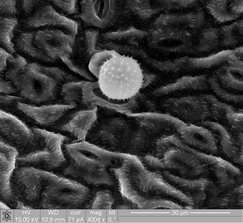
I am working with Australian Myrtaceae plants and investigating host responses to a newly arrived fungal pathogen, myrtle rust. Below is an electron scanning microscope image of a myrtle rust spore germinating on a eucalypt leaf made with the help of the Australian Microscopy & Microanalysis Research Facility (http://sydney.edu.au/acmm).

Just by way of some background, the pathogen has a very extensive Myrtaceae host-range and most Australian natural vegetation communities are composed of Myrtaceae plants. These include eucalypts, paperbark, bottle-brush, tea-tree, lemon-scented myrtle, waxflower and more…. The potential for devastating outbreaks under the right environmental conditions is therefore still a looming threat.

For my experiment I took leaf samples from 4 resistant  and 4 susceptible plants at three time points – pre-inoculation, 24 hours post inoculation and 48 hours post inoculation. I extracted and cleaned the RNA using commercial kits. I then made libraries of around 300 base pairs for paired-end Illumina sequencing on Hiseq2500. Two lanes for each sample were run. The raw data from these runs is where I will begin the bioinformatic explanation in my next post.